Introduction
Linear equations are equations of the form a1x1 + a2x2 + ... +
anxn = b, where a1...an are constants called coefficients,
x1...xn are variables, and b is the constant term. This equations is a linear
equation in n variables. The variables are also often seen as x, y, z, etc. Linear equations involve only
variables of degree 1 (no exponents or roots of the variables), and they involve only sums and constant
multiples of variables, without any products of variables.
The following equations are linear:
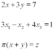
The following equations are NOT linear:

A solution of a linear equation is a vector composed of values [s1,...,sn], where when
we can substitute x1 = s1, ..., xn = sn to obtain a correct equation.
An equation in one variable (example, 2x = 6) has only one solution (a point on the real number line, in this case x = 6). A
linear equation in two variables has solutions which geometrically form a line in the plane. A linear
equation in three variables has solutions which form a plane. For linear equations of more variables, the
geometric interpretations aren't as clear, but they still have an infinite set of solutions.
Systems of linear equations are groups of more than one linear equation. Solving the system refers
to finding a solution common to all of the linear equations in the systems. There are only three
possibilities:
1) The system has one unique solution (a consistent system)
2) The system has infinitely many solutions (also a consistent system)
3) The system has no solutions (an inconsistent system)
Geometrically, one solution can be interpreted geometrically as the point where the various lines, planes, etc.
defined by the linear equations intersect. Infinitely many solutions occur when the equations define lines and/or planes
that intersect in a line or plane, such as the intersection of two planes or two equal lines. An inconsistent system
can be geometrically interpreted as lines and/or planes which never intersect, such as parallel lines in the plane, or
parallel lines or planes in 3 dimensions. In 3 dimensions, we can also have skew lines, which are not
parallel, but never intersect.
Methods of solving systems
When presented with a system of linear equations, we are almost always interested in solving that
system. Here, various methods of solving these systems are looked at, with important definitions and
theorems presented along the way. What is important to remember is that solving systems takes practice, and
several examples will be given.
Back substitution
Back substitution is the simplest method of finding the solution to the system, and is also the last
step in the more powerful methods of solving systems that we see later. Back substitution involves
isolating a single variable, and substituting it back into another equation to isolate another variable, and continuing
until we have solved for all variables.
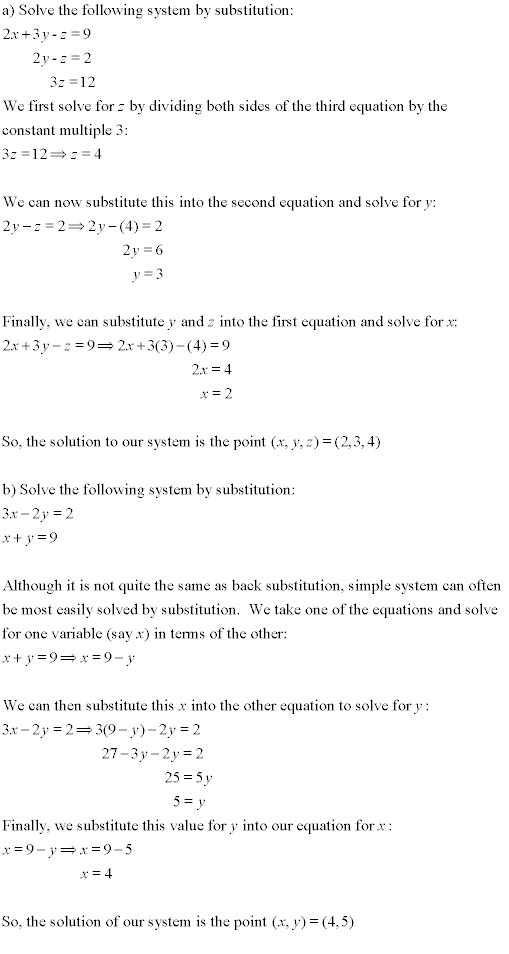
To use back substitution, we need a system like above where the a variable is already isolated, or
where we can express one variable in terms of another, as in the following example.
It is not often that our system of equations is already in a state where we can proceed directly to back
substitution. We need to get our system of equations to a point where we have isolated variables. We
can do this using elementary row operations. Elementary row operations can be used to change the system
to one that we can use back substitution on, without changing the solution. If we denote row 1 by R1,
row 2 by R2, etc., and k is a scalar, the three elementary row operations are
as follows:
1)Swap two rows (equations), denoted R1↔R2 (this would swap rows 1 and 2)
2)Multiply a row by a nonzero scalar, denoted kR1 (this would multiply row 1 by k)
3)Add a multiple of a row to another row, denoted R1 + kR2 (this would add k times row 2 to row 1, and replace the previous row 1)
Elementary row operations should be familiar from solving systems in high school math courses. By
introducing the concept of an augmented matrix, we can simplify our work on the system, and combine
this with elementary row operations and back substitution to define another method of solving systems.
(If matrices are not familiar to you, or you'd like to review the topic, see the
matrices tutorial) An augmented matrix is a matrix which contains the coefficients and constant terms from our
system of linear equations. By putting the systems in this matrix, we only need to concentrate on what
is important, these constants, since the variables themselves are never operated on. An augmented matrix
is as follows,

Gaussian Elimination
Gaussian elimination is a three step method for solving systems of linear equations:
1) Write out the system as an augmented matrix (use zeroes for a particular variable
of the system if it doesn't appear in one of the equations)
2) Use elementary row operations to reduce the matrix to row echelon form (see below)
3) Use back substitution to finally solve the system
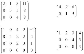
Row echelon form occurs when a matrix is in a form as follows:
1) The first entry in each row (called the leading entry) has only zeroes in the column
below it.
2) When a row has a leading entry, the leading entry in all rows above it are in columns to the left of
the leading entry.
The following matrices are in row echelon form:
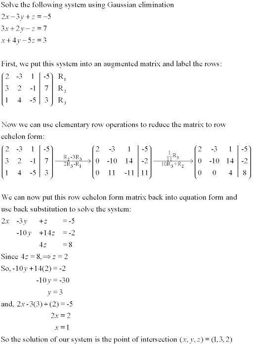
Let's take the system below and perform the steps involved in Gaussian elimination.

After putting the system into an augmented matrix, we perform elementary row operations on this system
until we get it into row echelon form as described above. This allows us to perform back substitution, beginning
with the bottom row in the system, in order to find the solution. In this way, Gaussian elimination provides
us with an algorithm of sorts to solve a system of linear equations. Below, we solve the above system using
Gaussian elimination.
Gauss-Jordan Elimination
We can improve the above method by adding another condition to Gaussian elimination. Gauss-Jordan elimination
involves the same steps as Gaussian elimination, but we continue elementary row operations until we get the
augmented matrix into row-reduced echelon form (rref), as defined next.
A matrix is in row-reduced echelon form if:
1) The leading entry in each row (if any) is a one.
2) There are no entries in the column above or below any leading entry.
3) Any leading entries in a row is to the right of a leading entry in a row above.
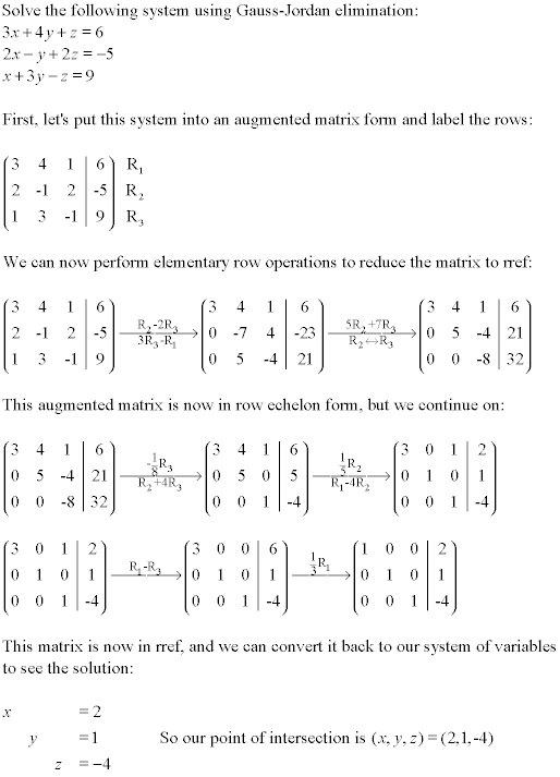
With Gauss-Jordan elimination, we avoid the need for back substitution. When our matrix is in rref, our leading
1's specify the variable in question, with our last column giving us the value for that variable. We specify a theorem
about rref before performing Gauss-Jordan elimination on a system below.
Theorem: The row-reduced echelon form of a matrix A, denoted by rref(A), is unique.
The rank of a matrix A, rank(A), is equal to the number of nonzero rows in rref(A). Using this information,
we can state the following theorem: The number of free variables in a system of linear
equations in n variables with augmented matrix A is found by the formula
number of free variables = n - rank(A)
Free variables are those not associated with a leading entry in the row echelon form of A, while those
with a leading entry are leading variables. When we have a consistent system with free variables, it means geometrically
that our lines or planes intersect in infinitely many places (a line or plane), rather than a single
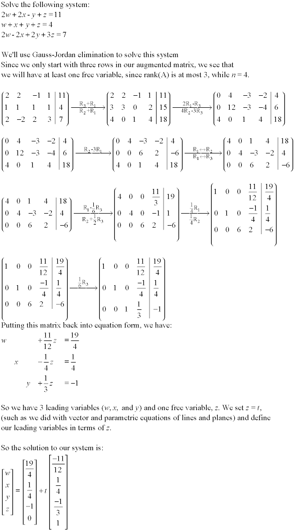
point. The free variables can be set to anything, and the leading variables depend on those free variables.
Let's see an example of this idea of free variables.
Homogeneous Systems
Homogeneous systems of linear equations are systems where the constant term in each equations is zero.
Therefore, they have the form [A|0], where A is the matrix of coefficients of the variables in the
system of equations. Systems of this type always have a solution. There is always the trivial solution where
[x1, x2, ..., xn] = [0,0,...0]. This can be interpreted as a point at
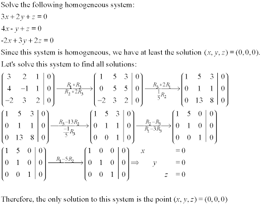
the origin of the space Rn. As well, the system may have infinitely many solutions. Let's
look at homogeneous systems.
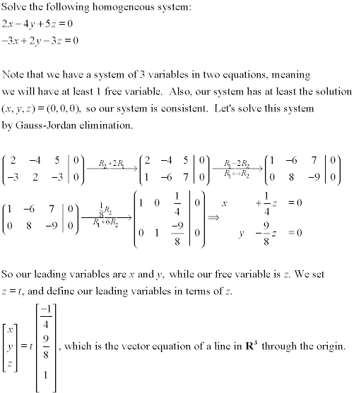
In a homogeneous system, if the number of equations is less than the number of variables in the system,
the system will always have infinitely many solutions. This is because a homogeneous system has to
be consistent, and our formula for free variables guarantees at least one free variable. Together, this
means that our homogeneous system will have infinitely many solutions, as shown below.
Linear Independence
A set of vectors is said to be linearly dependent if each vector in the set can be expressed
as a linear combination of the other ones. This is equivalent to saying that there is some nontrivial
linear combination (not all scalars are zero) of this set of vectors that equals 0. If the
vectors are not linearly dependent, they are otherwise called linearly independent. Solving
questions involving linear dependence involves putting our vectors into an augmented system, and then solving
that system. Some examples are below.
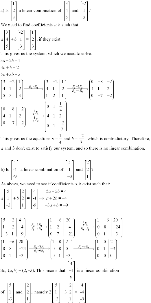
We can see from above that if a system of linear equations is put in augmented form [A|b], then
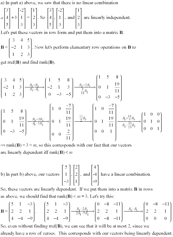
it has a solution if b is a linear combination of columns of A. Also, if we create a matrix B, where
the rows of B are vectors in row form, these vectors are linearly dependent iff (if and only if) Rank(B)<m, where m is
the number of vectors. Let's
take our above examples and show how this works.
Finally, any set of vectors in Rn is linearly dependent if the number of vectors (m) is greater than
the dimension of the space (n), that is, m>n.
Spanning Sets
Closely linked to the idea of linear dependence is the idea of spanning sets. Say we have a set of vectors in
Rn, where S = {v1, v2, ..., vk}. The set of
all possible linear combinations of the vectors in this set S is called the span of S. It is denoted
span(v1, v2, ..., vk) or span(S). If span(S) = Rn, then
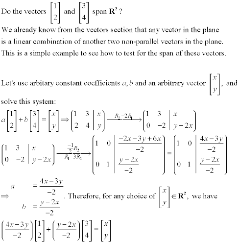
S is called a spanning set for Rn. S can also span subsets of the whole space, such
as a line, plane, etc. Let's look at an example of how to test to see if S is a spanning set.
Solving systems of linear equations can take some practice. Learning which methods are best and
learning how to correctly solve systems takes time, and more questions are provided in the sample
problems section of this site. You can also go to the test section
to see if and where you need to practice.
|
Top of Page |
|

